Excel Gantt Chart Template With Percentage Completion
Excel Gantt Chart Template with Percentage Completion: A Comprehensive Guide
Gantt charts are indispensable tools for project management, offering a visual representation of a project’s timeline, tasks, and dependencies. Integrating percentage completion into an Excel Gantt chart elevates its utility, providing a dynamic overview of progress and potential roadblocks. This guide delves into how to create and effectively use an Excel Gantt chart template with percentage completion tracking.
Understanding the Basics
A traditional Gantt chart typically comprises a list of tasks along the vertical axis and a timeline spanning the horizontal axis. Each task is represented by a bar whose length corresponds to its duration. Dependencies between tasks are often indicated by arrows or connecting lines. Adding percentage completion allows you to visualize how far along each task is, making it easier to identify tasks that are behind schedule or exceeding expectations.
Creating an Excel Gantt Chart Template
While Excel doesn’t have a built-in Gantt chart feature that automatically tracks percentage completion, you can easily create one using conditional formatting and formulas. Here’s a step-by-step approach:
1. Data Preparation
Start by creating a table with the following columns:
- Task Name: A descriptive name for each task.
- Start Date: The date the task is scheduled to begin.
- Duration (Days): The estimated number of days the task will take to complete.
- End Date (Calculated): This column will be calculated using a formula.
- Percentage Complete: A number between 0 and 1 (or 0% to 100%) representing the task’s completion status.
Populate the table with your project’s tasks, start dates, and durations. Use the following formula to calculate the End Date:
=Start Date + Duration - 1
This formula subtracts 1 because the start date is included in the duration.
2. Setting up the Chart Area
Create a separate area in your spreadsheet to serve as the Gantt chart itself. This area will consist of rows representing your tasks and columns representing dates.
- In the first row of your chart area, enter the start date of your project. In the cell to the right, use the following formula to increment the date by one day:
- Drag this formula across the row to create a series of dates that span the entire project duration.
- Format the date cells to display only the day of the month or a short date format to save space.
- In the first column of your chart area, list the task names from your data table.
=Previous Cell + 1
3. Conditional Formatting for Task Bars
This is where the magic happens. We’ll use conditional formatting to create the task bars based on the start date, end date, and percentage completion.
- Select the entire chart area (excluding the header row with dates and the first column with task names).
- Go to “Conditional Formatting” > “New Rule…”
- Choose “Use a formula to determine which cells to format.”
- Enter the following formula in the formula box (adjust cell references to match your spreadsheet):
COLUMN()returns the column number of the current cell being evaluated.MATCH($B2, $1:$1, 0)finds the column number of the Start Date for the current task (row 2). Adjust$B2to reference the correct Start Date column in your data table. Also, adjust$1:$1to match the row containing your dates in the chart area.MATCH($C2, $1:$1, 0)finds the column number of the End Date for the current task (row 2). Adjust$C2to reference the correct End Date column in your data table. Also, adjust$1:$1to match the row containing your dates in the chart area.AND()ensures that both conditions are met: the current column number is greater than or equal to the start date column number AND the current column number is less than or equal to the end date column number.- Click "Format..." and choose a fill color for the task bar. This represents the completed portion.
- Click "OK" to close the formatting dialogs.
=AND(COLUMN()>=MATCH($B2, $1:$1, 0), COLUMN()<=MATCH($C2, $1:$1, 0))
Explanation:
4. Conditional Formatting for Percentage Completion
Now, let's add the visual representation of percentage completion within the task bars.
- With the same chart area still selected, go to "Conditional Formatting" > "New Rule..."
- Choose "Use a formula to determine which cells to format."
- Enter the following formula (adjust cell references to match your spreadsheet):
- The first part,
COLUMN()>=MATCH($B2, $1:$1, 0), is the same as before, ensuring we're within the task's start date. $C2-$B2+1calculates the total duration of the task.($C2-$B2+1)*$E2multiplies the duration by the Percentage Complete (from column E).$B2+($C2-$B2+1)*$E2calculates the date corresponding to the completed percentage.MATCH($B2+($C2-$B2+1)*$E2, $1:$1, 0)finds the column number of the completed percentage date.- The entire formula ensures that only cells within the start date and the completed percentage date are formatted.
- Click "Format..." and choose a different fill color for the completed portion of the task bar. This color should visually indicate progress.
- Click "OK" to close the formatting dialogs.
=AND(COLUMN()>=MATCH($B2, $1:$1, 0), COLUMN()<=MATCH($B2+($C2-$B2+1)*$E2, $1:$1, 0))
Explanation:
5. Refining the Chart
- Gridlines: Consider removing gridlines for a cleaner look (View > Gridlines).
- Borders: Add borders to the chart area to visually separate it from the rest of the spreadsheet.
- Headers: Format the header row (dates) and the task name column for better readability. Freeze these panes to keep them visible as you scroll through the chart.
- Scaling: Adjust the column width to optimize the visual representation of the timeline.
Using the Gantt Chart Template
Once the template is set up, using it is straightforward:
- Enter your project tasks, start dates, and durations in the data table.
- Update the "Percentage Complete" column as tasks progress. The Gantt chart will automatically update to reflect the new completion status.
- Review the chart regularly to identify tasks that are behind schedule or require attention.
Advanced Tips
- Dependencies: Add a "Predecessor" column to indicate which tasks must be completed before others can start. Use formulas to automatically update start dates based on predecessor completion.
- Resources: Include columns for assigned resources and track resource allocation.
- Milestones: Highlight key milestones by using a different color or shape in the chart.
- Reporting: Create summary reports based on the Gantt chart data to track project progress and identify potential issues. Use pivot tables and charts for effective data visualization.
Conclusion
An Excel Gantt chart template with percentage completion is a powerful, accessible, and customizable tool for project management. By following these steps, you can create a dynamic visual representation of your project's timeline, track progress, and identify potential roadblocks, leading to more successful project outcomes. Remember to adapt the template to your specific project needs and regularly update the data to maintain an accurate and informative overview.
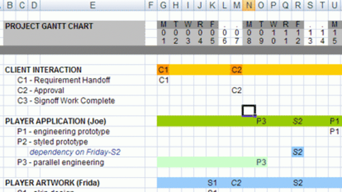 1200×675 excel gantt chart template gantt chart template pro vertex from db-excel.com
  0 x 0 gantt chart excel template teamgantt from www.teamgantt.com
 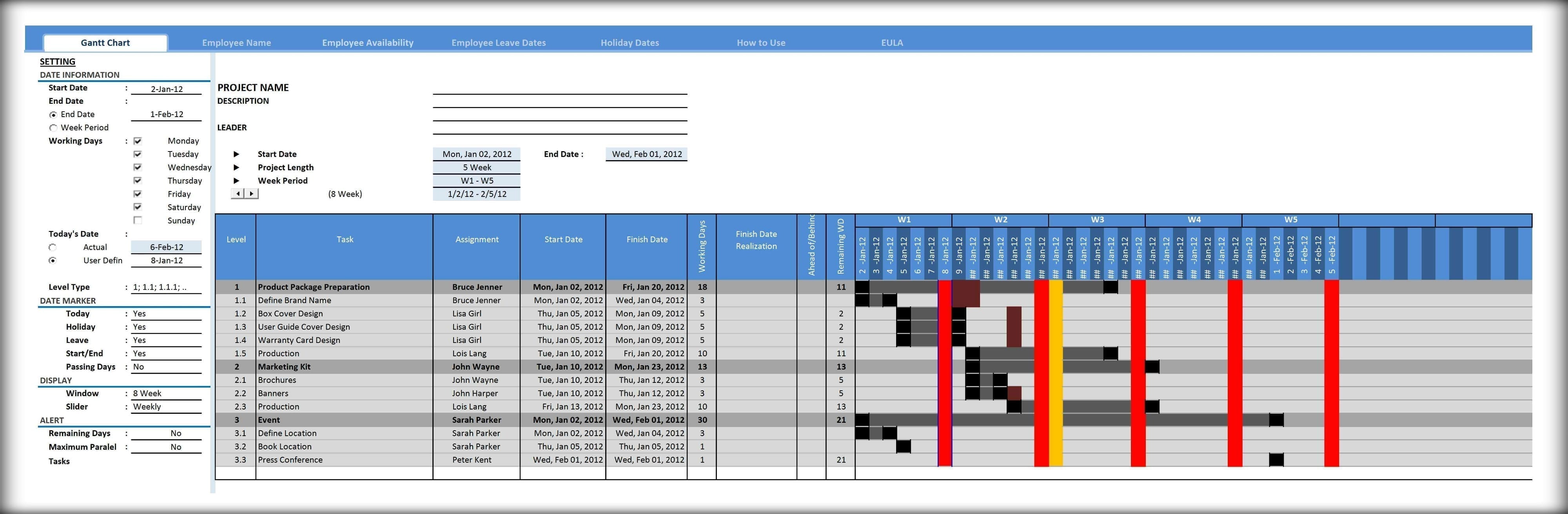 4000×1313 excel spreadsheet gantt chart template spreadsheet templates from excelxo.com
  1248×680 gantt chart template excel spreadshee gantt from db-excel.com
 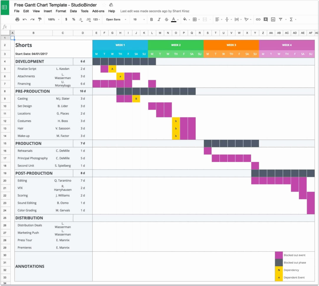 1082×970 gantt chart template excel spreadshee from db-excel.com
  1280×681 gantt chart excel template from www.engineeringmanagement.info
  1280×729 gantt chart template excel spreadshee from db-excel.com
 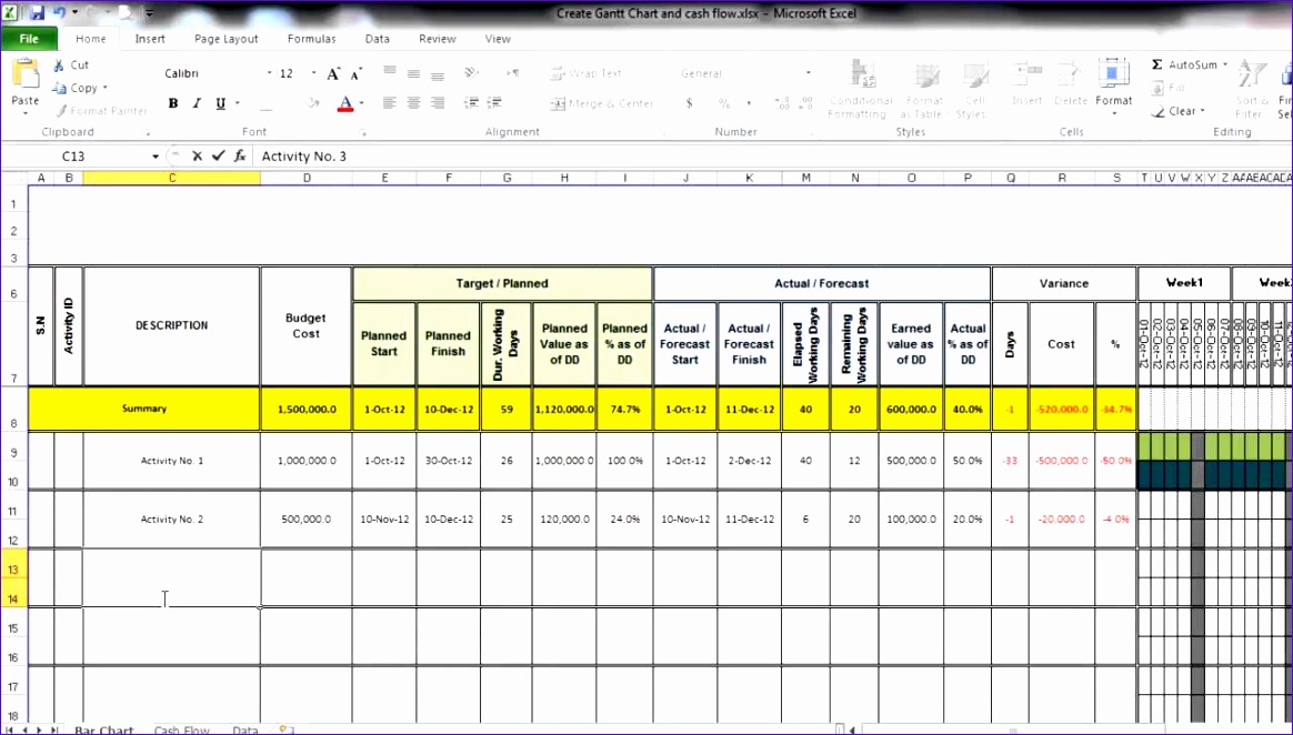 1164×662 excel spreadsheet gantt chart template excel templates from www.exceltemplate123.us
 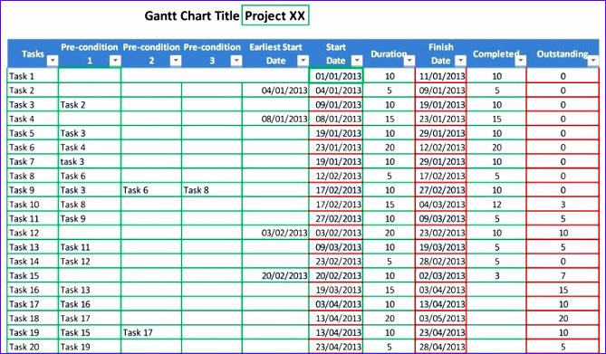 669×391 monthly gantt chart excel template excel templates from www.exceltemplate123.us
 Thank you for visiting Excel Gantt Chart Template With Percentage Completion. There are a lot of beautiful templates out there, but it can be easy to feel like a lot of the best cost a ridiculous amount of money, require special design. And if at this time you are looking for information and ideas regarding the Excel Gantt Chart Template With Percentage Completion then, you are in the perfect place. Get this Excel Gantt Chart Template With Percentage Completion for free here. We hope this post Excel Gantt Chart Template With Percentage Completion inspired you and help you what you are looking for.
Excel Gantt Chart Template With Percentage Completion was posted in December 5, 2025 at 1:11 pm. If you wanna have it as yours, please click the Pictures and you will go to click right mouse then Save Image As and Click Save and download the Excel Gantt Chart Template With Percentage Completion Picture.. Don’t forget to share this picture with others via Facebook, Twitter, Pinterest or other social medias! we do hope you'll get inspired by SampleTemplates123... Thanks again! If you have any DMCA issues on this post, please contact us!