Vertical Layout Gantt Chart Excel File
Creating a Vertical Layout Gantt Chart in Excel
Gantt charts are powerful tools for project management, providing a visual representation of project timelines, tasks, and dependencies. While the traditional horizontal layout is commonly used, a vertical layout Gantt chart can offer unique advantages, especially for projects with numerous tasks or a specific emphasis on task sequencing. This document explains how to create a functional and visually appealing vertical Gantt chart using Microsoft Excel.
Why Choose a Vertical Layout?
Before diving into the “how-to,” let’s consider the scenarios where a vertical Gantt chart might be preferable:
- Emphasis on Task Sequence: A vertical layout naturally emphasizes the order in which tasks are completed, making it easier to understand dependencies and critical path.
- Numerous Tasks: For projects with many small tasks, a vertical chart can be more manageable, allowing for better label visibility than a compressed horizontal chart.
- Unique Presentation Needs: A vertical layout offers a different visual perspective, which can be useful for presentations or reports where a fresh approach is desired.
Steps to Create a Vertical Gantt Chart in Excel
1. Data Preparation
The foundation of any Gantt chart is well-structured data. You’ll need the following columns:
- Task Name: A brief description of each task.
- Start Date: The date the task is scheduled to begin.
- Duration (Days): The number of days the task is expected to take. Alternatively, you could use an End Date column, calculating Duration later.
Here’s an example of how your data might look:
| Task Name | Start Date | Duration (Days) |
|---|---|---|
| Task 1: Project Planning | 1/1/2024 | 5 |
| Task 2: Requirements Gathering | 1/6/2024 | 7 |
| Task 3: Design Phase | 1/13/2024 | 10 |
| Task 4: Development | 1/23/2024 | 15 |
| Task 5: Testing | 2/7/2024 | 7 |
| Task 6: Deployment | 2/14/2024 | 3 |
2. Calculate End Date (If Necessary)
If you only have Start Date and Duration, add a column called “End Date” and use the following formula in the first cell of the column (assuming Start Date is in column B and Duration is in column C):
=B2+C2-1
Copy this formula down to calculate the End Date for all tasks. Subtracting ‘1’ ensures the end date is inclusive of the start date.
3. Determine the Chart’s Date Range
You need to determine the overall start and end dates for your project to establish the chart’s timeframe. Use the following formulas:
- Project Start Date:
=MIN(B:B)(assuming Start Date is in column B) - Project End Date:
=MAX(D:D)(assuming End Date is in column D)
4. Create a Helper Table for the Chart
This is the crucial step for creating a vertical Gantt chart. You’ll create a table where dates are listed vertically, and tasks are listed horizontally. This table will form the basis of your chart.
- List Dates Vertically: In a new sheet (or a separate section of your current sheet), in cell A1, enter the Project Start Date. In cell A2, enter the formula:
=A1+1. Copy this formula down until you reach the Project End Date. You can check if you’ve reached the end date by ensuring the last date in the list matches the Project End Date calculated earlier. You can also drag the little square at the bottom right of the cell downwards until you get to the correct date. - List Tasks Horizontally: In the first row (row 1), starting from column B, list the names of your tasks.
- Populate the Table with Logic: This is where the Gantt chart magic happens. In cell B2, enter the following formula (adjust the cell references to match your data):
=IF(AND($A2>=Sheet1!$B2, $A2<=Sheet1!$D2),1,0)This formula checks if the date in column A falls within the Start Date and End Date range for the task listed in row 1. If it does, it displays a "1"; otherwise, it displays a "0." `Sheet1` is assumed to be the sheet where the initial data table resides. Ensure the sheet name and cell references are accurate for your data. Use dollar signs ($) to lock the column and row references as shown. So `$A2` will always refer to column A, but the row will change. `Sheet1!$B2` will always refer to the start date of the first task in Sheet1.
- Copy the Formula: Copy the formula in cell B2 to all the other cells in the table. This will populate the table with 1s and 0s, indicating when each task is active. Drag the little square on the bottom right of the cell both downwards and sideways.
5. Create the Chart
- Select the Data: Select the entire helper table, including the dates and task names.
- Insert a Stacked Bar Chart: Go to the "Insert" tab in Excel and choose a "Stacked Bar Chart." This chart type is essential for creating the visual representation of the Gantt chart.
- Rotate the Chart: Right-click on the chart area and select "Format Chart Area." In the Format Chart Area pane, go to "Size & Properties" and find "Alignment." Change the text direction to rotate the chart 90 degrees counter-clockwise. This will effectively create the vertical layout.
6. Format the Chart
The initial chart will likely need formatting to improve its readability and visual appeal:
- Remove the First Series (Dates): The first data series (representing the dates) is currently visible as a colored bar. Select this series by clicking on it in the chart, and then go to "Format Data Series." Set the "Fill" to "No Fill." This will hide the date series, leaving only the bars representing the tasks.
- Adjust Axis Labels: Format the vertical (task name) axis to display task names clearly. Rotate the labels if necessary. Format the horizontal (date) axis to display dates in a readable format.
- Add Gridlines (Optional): Adding horizontal gridlines can improve readability by helping to visually align tasks with specific dates.
- Customize Colors: Change the colors of the bars to differentiate tasks or to match your branding.
- Add a Chart Title and Axis Labels: Clearly label the chart and axes to provide context and improve understanding.
Tips and Tricks
- Conditional Formatting: Use conditional formatting in your helper table to visually highlight critical dates or tasks based on their progress.
- Error Handling: Implement error handling in your formulas to prevent unexpected results if the data contains errors.
- Dynamic Updates: Make your chart dynamic by using named ranges and formulas to automatically update the chart when the data changes.
- Excel Templates: Consider creating an Excel template to easily create vertical Gantt charts for future projects.
By following these steps and tips, you can effectively create a vertical layout Gantt chart in Excel, providing a clear and informative visualization of your project timeline.
 655×320 glossy gantt chart vertical microsoft excel undefined from www.officetooltips.com
  1280×577 create gantt chart excel ganttxl from ganttxl.com
  1434×442 create gantt chart excel from smartsheet.com
  1300×800 gantt charts excel templates tutorial video smartsheet from smartsheet.com
  2052×772 create gantt chart excel smartsheet from www.smartsheet.com
 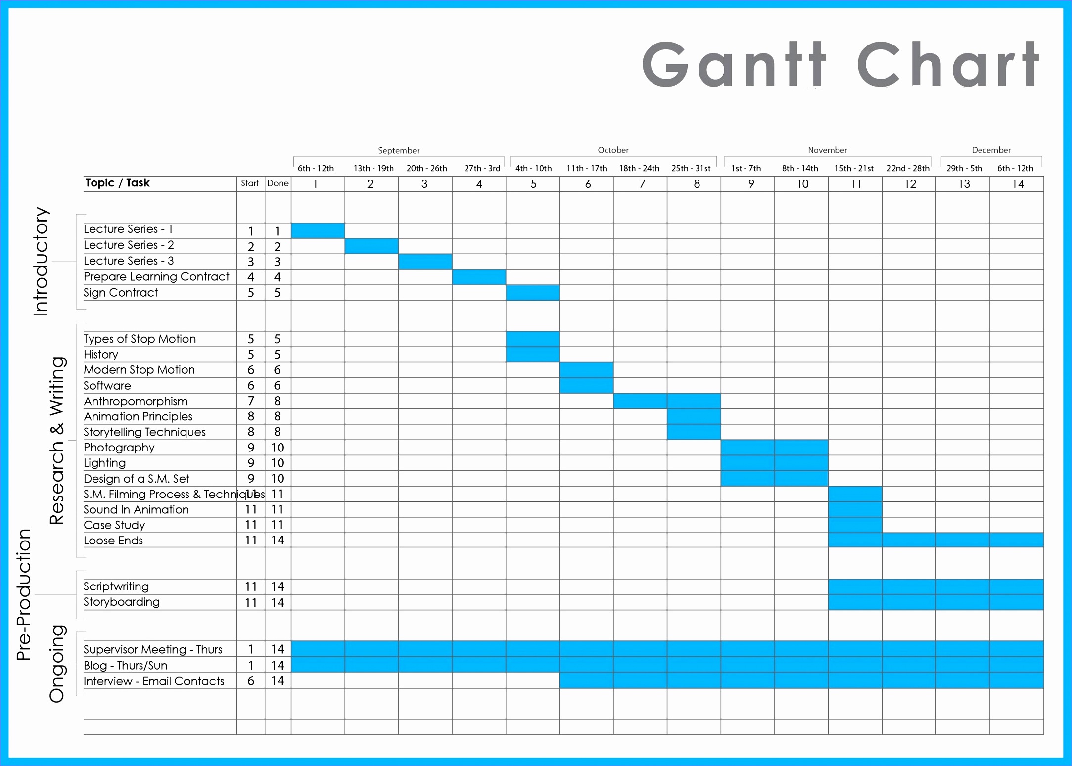 2167×1549 gantt chart templates excel excel templates from www.exceltemplate123.us
  1900×929 create gantt chart complete functionality excel from gyankosh.net
 Thank you for visiting Vertical Layout Gantt Chart Excel File. There are a lot of beautiful templates out there, but it can be easy to feel like a lot of the best cost a ridiculous amount of money, require special design. And if at this time you are looking for information and ideas regarding the Vertical Layout Gantt Chart Excel File then, you are in the perfect place. Get this Vertical Layout Gantt Chart Excel File for free here. We hope this post Vertical Layout Gantt Chart Excel File inspired you and help you what you are looking for.
Vertical Layout Gantt Chart Excel File was posted in August 17, 2025 at 10:54 am. If you wanna have it as yours, please click the Pictures and you will go to click right mouse then Save Image As and Click Save and download the Vertical Layout Gantt Chart Excel File Picture.. Don’t forget to share this picture with others via Facebook, Twitter, Pinterest or other social medias! we do hope you'll get inspired by SampleTemplates123... Thanks again! If you have any DMCA issues on this post, please contact us!